Video Game Sales Dataset Descriptive Analysis
About Data Set:
About Dataset This dataset provides a comprehensive list of video games with sales exceeding 100,000 copies. The data was collected through web scraping from vgchartz.com, ensuring a robust compilation of sales figures for various games across multiple regions and platforms.
Key Features of the Dataset: Rank: Indicates the global sales ranking of each game. Name: Specifies the title of the game. Platform: Identifies the platform on which the game was released (e.g., PC, PS4, Xbox One). Year: Records the year of the game's release. Genre: Categorizes the game based on its genre (e.g., Action, Adventure, RPG). Publisher: Lists the company responsible for publishing the game. Regional Sales Data: NA_Sales: Sales in North America, measured in millions. EU_Sales: Sales in Europe, measured in millions. JP_Sales: Sales in Japan, measured in millions. Other_Sales: Sales in the rest of the world, measured in millions. Global_Sales: Represents the total worldwide sales, aggregating all regional sales. The dataset contains 16,598 records, offering a rich resource for analysis. Notably, two entries were excluded due to incomplete information.
Data Collection Method: The dataset was generated using a Python script available on GitHub. The script utilizes the BeautifulSoup library for web scraping, ensuring accurate and detailed extraction of data.
This dataset is an invaluable resource for analyzing video game sales trends, evaluating the performance of specific platforms or genres, and understanding regional preferences in the gaming industry.
Step 1: Data Wrangling
#Importing essential libraries
import pandas as pd
import numpy as np
import matplotlib.pyplot as plt
import seaborn as sns
import warnings
warnings.filterwarnings("ignore", category=FutureWarning)
#Viewing Our DataFrame!
df = pd.read_csv("vgsales new.csv")
df.head()
| Rank | Name | Platform | Year | Genre | Publisher | NA_Sales | EU_Sales | JP_Sales | Other_Sales | Global_Sales | |
|---|---|---|---|---|---|---|---|---|---|---|---|
| 0 | 259 | Asteroids | 2600 | 1980.0 | Shooter | Atari | 4.00 | 0.26 | 0.0 | 0.05 | 4.31 |
| 1 | 545 | Missile Command | 2600 | 1980.0 | Shooter | Atari | 2.56 | 0.17 | 0.0 | 0.03 | 2.76 |
| 2 | 1768 | Kaboom! | 2600 | 1980.0 | Misc | Activision | 1.07 | 0.07 | 0.0 | 0.01 | 1.15 |
| 3 | 1971 | Defender | 2600 | 1980.0 | Misc | Atari | 0.99 | 0.05 | 0.0 | 0.01 | 1.05 |
| 4 | 2671 | Boxing | 2600 | 1980.0 | Fighting | Activision | 0.72 | 0.04 | 0.0 | 0.01 | 0.77 |
# 1. Check for missing values
print(df.isnull().sum())
Rank              0
Name              0
Platform          0
Year            271
Genre             0
Publisher        58
NA_Sales          0
EU_Sales          0
JP_Sales          0
Other_Sales       0
Global_Sales      0
dtype: int64
# 2. Drop missing values
df.dropna(inplace=True)
print(df.isnull().sum())
Rank            0
Name            0
Platform        0
Year            0
Genre           0
Publisher       0
NA_Sales        0
EU_Sales        0
JP_Sales        0
Other_Sales     0
Global_Sales    0
dtype: int64
# 3. Check for duplicates
print(df.duplicated().sum())
0
# 4. Check data types
print(df.dtypes)
Rank              int64
Name             object
Platform         object
Year            float64
Genre            object
Publisher        object
NA_Sales        float64
EU_Sales        float64
JP_Sales        float64
Other_Sales     float64
Global_Sales    float64
dtype: object
# 5. Check the shape of the DataFrame
df.shape
(16291, 11)
# 6. Concise summary of the DataFrame
df.info()
<class 'pandas.core.frame.DataFrame'>
Index: 16291 entries, 0 to 16326
Data columns (total 11 columns):
 #   Column        Non-Null Count  Dtype
---  ------        --------------  -----
 0   Rank          16291 non-null  int64
 1   Name          16291 non-null  object
 2   Platform      16291 non-null  object
 3   Year          16291 non-null  float64
 4   Genre         16291 non-null  object
 5   Publisher     16291 non-null  object
 6   NA_Sales      16291 non-null  float64
 7   EU_Sales      16291 non-null  float64
 8   JP_Sales      16291 non-null  float64
 9   Other_Sales   16291 non-null  float64
 10  Global_Sales  16291 non-null  float64
dtypes: float64(6), int64(1), object(4)
memory usage: 1.5+ MB
# 7. Change 'Year' from float to integer
df['Year'] = df['Year'].astype(int)
# 8. Concise summary of the DataFrame  after changing the data type
df.info()
<class 'pandas.core.frame.DataFrame'>
Index: 16291 entries, 0 to 16326
Data columns (total 11 columns):
 #   Column        Non-Null Count  Dtype
---  ------        --------------  -----
 0   Rank          16291 non-null  int64
 1   Name          16291 non-null  object
 2   Platform      16291 non-null  object
 3   Year          16291 non-null  int32
 4   Genre         16291 non-null  object
 5   Publisher     16291 non-null  object
 6   NA_Sales      16291 non-null  float64
 7   EU_Sales      16291 non-null  float64
 8   JP_Sales      16291 non-null  float64
 9   Other_Sales   16291 non-null  float64
 10  Global_Sales  16291 non-null  float64
dtypes: float64(5), int32(1), int64(1), object(4)
memory usage: 1.4+ MB
# Optional: Export the cleaned DataFrame to a CSV file, used to also demonstrate data visualisation in other software such as Tableau, Power BI, etc.
#df.to_csv('vgsales_clean.csv', index=False)

#print("DataFrame exported successfully.")
Step 2: Exploratory Data Aanalysis
# 9. Display summary statistics
print(df.describe())
               Rank          Year      NA_Sales      EU_Sales      JP_Sales  \
count  16291.000000  16291.000000  16291.000000  16291.000000  16291.000000
mean    8290.190228   2006.405561      0.265647      0.147731      0.078833
std     4792.654450      5.832412      0.822432      0.509303      0.311879
min        1.000000   1980.000000      0.000000      0.000000      0.000000
25%     4132.500000   2003.000000      0.000000      0.000000      0.000000
50%     8292.000000   2007.000000      0.080000      0.020000      0.000000
75%    12439.500000   2010.000000      0.240000      0.110000      0.040000
max    16600.000000   2020.000000     41.490000     29.020000     10.220000

        Other_Sales  Global_Sales
count  16291.000000  16291.000000
mean       0.048426      0.540910
std        0.190083      1.567345
min        0.000000      0.010000
25%        0.000000      0.060000
50%        0.010000      0.170000
75%        0.040000      0.480000
max       10.570000     82.740000
Description
- Rank
Count: 16,291 (all data points are present). Mean: 8,290.2 (average rank is near the middle of the range). Standard Deviation (std): 4,792.7 (ranks are widely dispersed). Minimum (min): 1 (highest-ranked game). 25th Percentile (25%): 4,132.5 (25% of games are ranked 4,132 or lower). Median (50%): 8,292 (middle rank of the dataset). 75th Percentile (75%): 12,439.5 (75% of games are ranked 12,439 or lower). Maximum (max): 16,600 (lowest-ranked game). Insights: Ranks are evenly distributed, and the median is close to the mean, suggesting no strong skew.
- Year
Count: 16,291. Mean: 2006.4 (most games were released around 2006). Standard Deviation: 5.8 (release years are slightly spread out). Min: 1980 (oldest game in the dataset). 25%: 2003 (25% of games were released before 2003). Median: 2007. 75%: 2010 (75% of games were released before 2010). Max: 2020 (most recent game). Insights: The majority of games are concentrated between 2003 and 2010, with a few older and newer games.
- NA_Sales (North America Sales)
Mean: 0.27 (average sales are relatively low). Std: 0.82 (high variability in sales). Min: 0 (some games had no sales). 25%: 0 (25% of games had no sales in North America). Median: 0.08 (50% of games sold less than 0.08 units). 75%: 0.24 (75% of games sold less than 0.24 units). Max: 41.49 (best-selling game sold 41.49 units). Insights: NA_Sales is heavily right-skewed, with most games selling very few units and a few outliers with extremely high sales.
- EU_Sales (Europe Sales)
Mean: 0.15 (average sales are even lower than NA_Sales). Std: 0.51 (moderate variability). Min: 0 (some games had no sales in Europe). 25%: 0 (25% of games had no sales in Europe). Median: 0.02 (50% of games sold less than 0.02 units). 75%: 0.11 (75% of games sold less than 0.11 units). Max: 29.02 (best-selling game sold 29.02 units). Insights: Like NA_Sales, EU_Sales is also highly skewed, with a few games achieving significant sales.
- JP_Sales (Japan Sales)
Mean: 0.08 (average sales are very low). Std: 0.31 (less variability compared to NA_Sales and EU_Sales). Min: 0 (some games had no sales in Japan). 25%: 0 (25% of games had no sales in Japan). Median: 0 (50% of games sold no units in Japan). 75%: 0.04 (75% of games sold less than 0.04 units). Max: 10.22 (best-selling game sold 10.22 units). Insights: Sales in Japan are very low for most games, with few exceptions.
- Other_Sales
Mean: 0.05 (average sales are minimal). Std: 0.19 (low variability). Min: 0 (some games had no sales in other regions). 25%: 0 (25% of games had no sales in other regions). Median: 0.01 (50% of games sold less than 0.01 units). 75%: 0.04 (75% of games sold less than 0.04 units). Max: 10.57 (best-selling game sold 10.57 units). Insights: Sales in other regions are mostly negligible, with very few games achieving notable sales.
- Global_Sales
Mean: 0.54 (average sales are higher than any individual region). Std: 1.57 (significant variability). Min: 0.01 (some games barely sold globally). 25%: 0.06 (25% of games sold less than 0.06 units globally). Median: 0.17 (50% of games sold less than 0.17 units globally). 75%: 0.48 (75% of games sold less than 0.48 units globally). Max: 82.74 (best-selling game sold 82.74 units globally). Insights: Global_Sales aggregates all regions, showing a more pronounced right skew due to a few blockbuster games with extremely high sales.
Overall Insights:
Skewed Sales Data: Sales are heavily skewed across all regions, with the majority of games having very low sales and a few outliers with extremely high sales.
Regional Differences: North America has the highest average sales, followed by Europe, Japan, and other regions.
Time Period: Most games in the dataset were released between 2003 and 2010.
Global Perspective: A few games dominate the market, as indicated by the high maximum global sales compared to the mean and median.
# 10. Display data distribution
# Histograms
df.hist(bins=30, figsize=(15, 10))
plt.show()

My Tableau Visualization
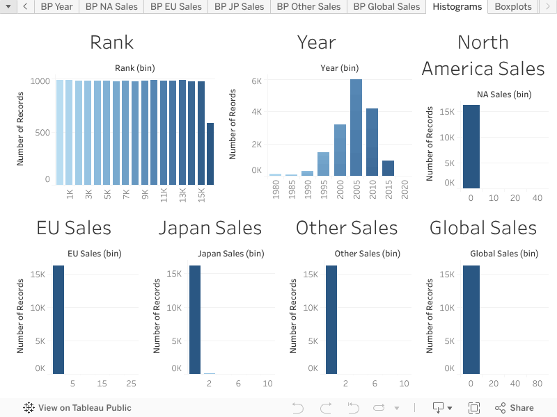
Description of each histogram
- Rank
The Rank histogram shows a nearly uniform distribution of rank values. It suggests that rank values are distributed fairly evenly across the dataset. 2. Year The Year histogram shows a significant concentration of data around the years 2005–2015. This indicates that the dataset likely contains the majority of its data points from this period. 3. NA_Sales The NA_Sales histogram is highly skewed to the right, with most data concentrated around low sales values. A few outliers may exist with significantly higher sales values. 4. EU_Sales The EU_Sales histogram follows a similar pattern to NA_Sales, with most data points concentrated around low sales values. Again, a few higher sales outliers are present. 5. JP_Sales The JP_Sales histogram also shows a right-skewed distribution with most sales values near zero. There are very few higher sales points, suggesting lower sales volume in Japan compared to other regions. 6. Other_Sales The Other_Sales histogram has a similar right-skewed pattern, with most values concentrated around the lower end. It suggests minimal sales in other regions with rare higher values. 7. Global_Sales The Global_Sales histogram exhibits a right-skewed distribution, indicating that most games have low global sales. There are a few outliers with extremely high global sales.
Key Observations:
- Right-Skewed Distributions:
Sales data (NA_Sales, EU_Sales, JP_Sales, Other_Sales, and Global_Sales) all show right-skewed distributions, meaning that most values are small, with only a few larger values (outliers).
- Time Concentration:
Most data points for the Year column fall between 2005 and 2015, likely reflecting a period of high activity or data availability.
- Rank Distribution:
The Rank column is more uniformly distributed compared to the sales data. This suggests that the dataset focuses heavily on sales data from a specific period (2005–2015), with significant differences in sales volumes across regions.
# Boxplots
df.plot(kind='box', subplots=True, layout=(3, 3), figsize=(15, 10))
plt.show()

My Tableau Visualization
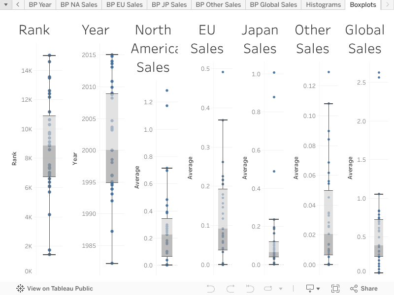
Description of each histogram
- Rank
The Rank boxplot shows a relatively wide interquartile range (IQR), suggesting a uniform distribution of rank values. There are no apparent outliers, as all data points lie within the whiskers. 2. Year The Year boxplot has most of its data concentrated between the mid-1990s and early 2010s. There are several outliers below the lower whisker, representing data points from earlier years (before 1990). 3. NA_Sales The NA_Sales boxplot is highly skewed with a small IQR near zero, indicating that most sales in North America are low. Numerous outliers above the upper whisker represent games with significantly high sales, exceeding 10 or even 30 units (possibly in millions). 4. EU_Sales The EU_Sales boxplot is similar to NA_Sales, with a small IQR and most values close to zero. Outliers exist above the upper whisker, showing a few games with higher sales in Europe, up to around 25 units. 5. JP_Sales The JP_Sales boxplot also has a small IQR near zero, reflecting low sales in Japan for most games. A few outliers exceed the upper whisker, with sales reaching up to 10 units for a small number of games. 6. Other_Sales The Other_Sales boxplot displays a similar pattern to the regional sales columns, with most sales close to zero and a small IQR. There are a few outliers representing higher sales in other regions, up to about 10 units. 7. Global_Sales The Global_Sales boxplot combines data from all regions, resulting in a larger IQR but still concentrated near zero. There are several extreme outliers above the upper whisker, with global sales reaching up to 80 units for a small subset of games.
Key Observations:
- Right-Skewed Distributions:
All sales columns (NA_Sales, EU_Sales, JP_Sales, Other_Sales, and Global_Sales) are heavily skewed toward lower values, with many outliers indicating games with significantly higher sales.
- Outliers:
Sales columns contain numerous outliers, representing games with exceptional performance in terms of sales.
- Year Outliers:
The Year column has outliers for older games (pre-1990), suggesting the dataset contains data from a wide range of release years.
- Rank Uniformity:
The Rank column appears to have no significant outliers, indicating a relatively even distribution of ranks. These boxplots provide a clear view of the central tendency, variability, and outliers for each column in the dataset.
# 11. Correlation matrix
# Select only numeric columns
numeric_df = df.select_dtypes(include=[np.number])

# Compute the correlation matrix
corr = numeric_df.corr()

# Plot the correlation matrix
sns.heatmap(corr, annot=True, cmap='coolwarm')
plt.show()

Color Scale
The color scale ranges from -1 (dark blue) to 1 (dark red):
- 1 (dark red): Perfect positive correlation.
- -1 (dark blue): Perfect negative correlation.
- 0 (white): No correlation.
Key Observations:
Rank
- Rank vs Global_Sales (-0.43):
- Negative correlation indicates that better-ranked games (lower rank values) tend to have higher global sales.
- Rank vs NA_Sales, EU_Sales, JP_Sales, and Other_Sales (around -0.27 to -0.40):
- Negative correlations suggest that better-ranked games tend to perform well in all regions.
- Rank vs Year (0.18):
- Weak positive correlation suggests that rank slightly improves for more recent games.
Year
- Year vs Global_Sales (-0.075):
- Very weak negative correlation, meaning the release year doesn't strongly influence global sales.
- Year vs Regional Sales (close to 0):
- Release year has negligible correlation with sales in individual regions.
NA_Sales
- NA_Sales vs Global_Sales (0.94):
- Very strong positive correlation, indicating North American sales contribute significantly to global sales.
- NA_Sales vs EU_Sales (0.77):
- Strong positive correlation, suggesting that games successful in North America often perform well in Europe.
- NA_Sales vs Other_Sales (0.63):
- Moderate positive correlation with sales in other regions.
- NA_Sales vs JP_Sales (0.45):
- Moderate correlation, indicating less overlap between sales success in North America and Japan.
EU_Sales
- EU_Sales vs Global_Sales (0.90):
- Very strong positive correlation, showing European sales are a significant contributor to global sales.
- EU_Sales vs Other_Sales (0.73):
- Strong correlation with sales in other regions.
- EU_Sales vs JP_Sales (0.44):
- Moderate correlation, indicating some alignment between sales success in Europe and Japan.
JP_Sales
- JP_Sales vs Global_Sales (0.61):
- Moderate positive correlation, showing that Japan contributes to global sales, but less so than North America or Europe.
- JP_Sales vs Other_Sales (0.29):
- Weak correlation, indicating limited overlap in sales trends between Japan and other regions.
Other_Sales
- Other_Sales vs Global_Sales (0.75):
- Strong positive correlation, indicating other regional sales significantly contribute to global sales.
- Other_Sales vs Regional Sales (NA, EU, JP):
- Moderate correlations, suggesting some overlap in sales patterns across regions.
Global_Sales
- Global_Sales vs Regional Sales:
- Very strong correlations with NA_Sales (0.94), EU_Sales (0.90), and Other_Sales (0.75).
- Moderate correlation with JP_Sales (0.61), reflecting Japan's relatively smaller contribution to global sales.
General Insights
-
Global Sales Drivers:
- North American and European sales have the strongest correlations with global sales.
- Japan and other regions have weaker contributions to global sales compared to NA and EU.
-
Regional Sales Alignment:
- NA_Sales and EU_Sales have the strongest alignment, indicating that games successful in one region are often successful in the other.
- Japan shows weaker alignment with other regions, reflecting distinct market dynamics.
-
Rank Correlations:
- Negative correlations with sales indicate that better-ranked games tend to sell more globally and regionally.
-
Year Impact:
- Release year has minimal impact on sales, suggesting other factors are more critical to a game's success.
- This correlation matrix helps identify relationships between sales in different regions and their contribution to global performance.
This correlation matrix helps identify relationships between sales in different regions and their contribution to global performance.
# 12. Pairplot
sns.pairplot(df)
plt.show()

1. Diagonal Plots (Histograms)
- The diagonal contains histograms for individual variables, showing their distribution.
- Rank: A relatively uniform distribution with many games spread across the rank range.
- Year: Most games are concentrated between 2000 and 2015.
- NA_Sales, EU_Sales, JP_Sales, Other_Sales, Global_Sales: All exhibit heavily right-skewed distributions, with most sales concentrated near zero and a few outliers with high sales.
2. Scatterplots (Off-Diagonal Plots)
The off-diagonal plots show scatterplots of the relationships between pairs of variables:
Rank vs Sales (NA_Sales, EU_Sales, JP_Sales, Other_Sales, Global_Sales)
- There is a clear negative trend: better-ranked games (lower rank) tend to have higher sales across all regions and globally.
- The scatterplots are dense at the lower sales levels, with outliers showing games with exceptionally high sales.
Year vs Sales
- There is no strong pattern between release year and sales. However:
- A slight increase in sales is observed for games released in the early 2000s to early 2010s.
- Sales for older games (pre-1990) and recent games (post-2015) are sparse and lower.
Regional Sales vs Global Sales
- NA_Sales, EU_Sales, JP_Sales, and Other_Sales vs Global_Sales:
- Strong positive linear relationships, especially for North America and Europe, indicating that these regions contribute significantly to global sales.
- Japan's sales show a weaker positive trend compared to other regions.
Regional Sales vs Each Other
- NA_Sales vs EU_Sales: Strong positive trend; games that sell well in North America often perform well in Europe.
- NA_Sales vs JP_Sales / EU_Sales vs JP_Sales: Moderate trends; sales success in North America and Europe is less aligned with Japan.
- Other_Sales vs NA_Sales / EU_Sales: Moderate positive relationships; some correlation exists between these regions and "other" sales.
Key Insights
- Rank as a Predictor of Sales:
- Lower (better) ranks are strongly associated with higher sales globally and in all regions.
- Outliers with very high sales are better ranked.
- Sales Distributions:
- Sales data is heavily skewed, with the majority of games having low sales and a few top-selling games contributing disproportionately.
- Global and Regional Sales Correlations:
- North America and Europe are the strongest contributors to global sales.
- Japan has less alignment with other regions, indicating distinct market preferences.
- Time Trends:
- The dataset contains most games between 2000 and 2015, with fewer games before 1990 or after 2015.
- Sales show minimal dependency on release year, though most high-sales games were released in the early 2000s to early 2010s.
Overall
This pairplot highlights the relationships between variables, confirming:- Strong correlations between global and regional sales.
- A negative relationship between rank and sales.
- Skewed distributions across sales metrics.